PHash Blog
perceptual hashing information
On Extracting Concise Image Descriptors from Natural Images
07 Apr 2019 - by starkdg
Image descriptors are essential for organizing a collection of images for the purpose
of search and retrieval. These can be as simple as unique file names, where an exact
file name is needed to retrieve each and every source image. In order to preserve a
sense of distance between images, however, where smaller distance indicate similarity and larger
distances wholy different images, a more elaborate scheme is necessary. The descriptors
need to preserve some of the essential features of the source image.
As is well known by now, convolutional neural networks can be trained to give good performance on image classification tasks. Several models perform at or above 95% classification accuracy (tf-slim). These neural networks are many layers deep. They take an image as input and output an indication as to which class among many is most probable. Interestingly, new classification layers can be fine-tuned on top of the model’s hidden layers and achieve comparable performance on new classification tasks. This suggests that the network’s hidden layers have learned fundamental features of the images. Furthermore, the outputs from these hidden layers can serve as quality descriptors, which preserve smoothness with subtle changes in input. However, they still exist in a relatively high dimensional feature space, making it difficult for fast indexing.
This post explores the cross correlations in these hidden layer values - also called feature vectors - in the hopes of reducing its size. It is our expectation that concise descriptors can be extracted from these feature vectors with the minimal additional overhead of training a few extra layers that can piggy-back on top of these classification models.
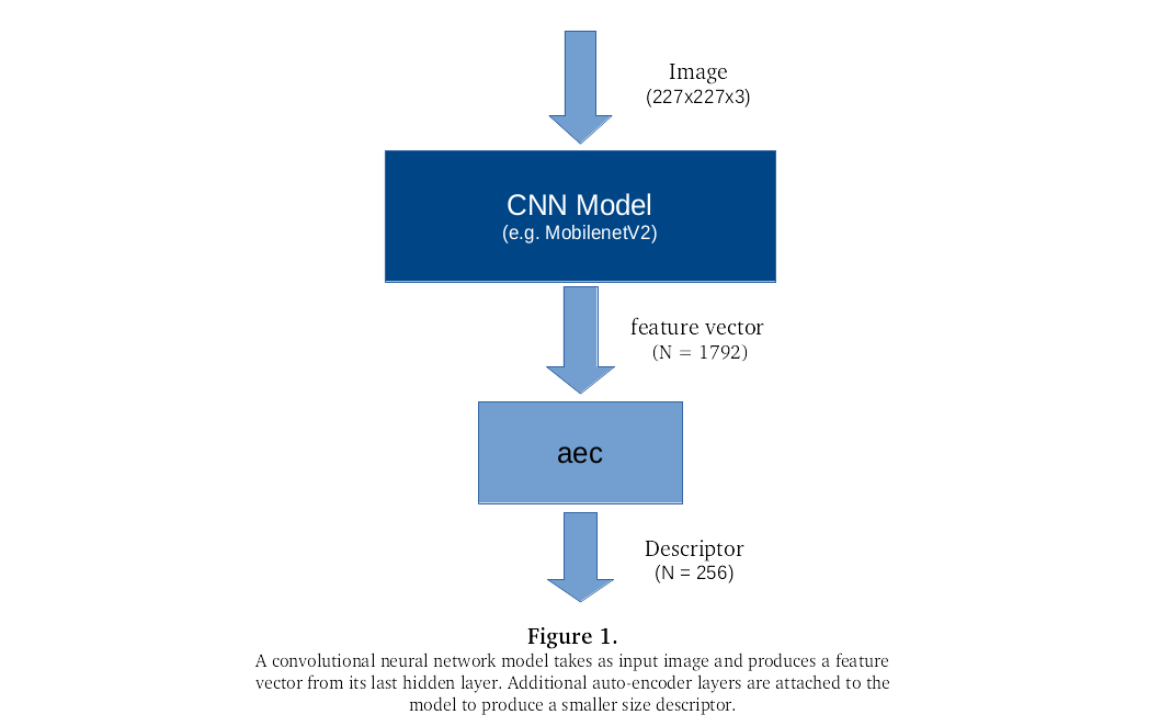
Here’s the general idea:
Objectives For This Post:
-
The development of a concise image descriptor suitable for long-term storage. It should be robust enough for fast comparison using a distance metric - like euclidean distance. This metric should preserve small distances for perceptually similar images, while keeping wholely unique images far enough apart.
-
Provide some fresh insight into the topology of these models’ feature vectors. Together with the right kind of indexing structure, we should be able to retrieve all nearest neighbors of a given image and get a good visual indication for what similar means in terms of the model’s feature vector. We will use the MobilenetV2 neural net for all our work, but all the code is easy to modify to explore other models.
-
Develop a testing framework to evaluate these descriptors for this application. This framework can be used to test the descriptors as well as the feature vector itself. In this way, we will be able to see just where the descriptors lose the ability to discriminate between images as well as compare the effectiveness of the new descriptors.
All code can be found in the github repository here: View On GitHub
A Test Framework
We need a framework to test all our models. First, we start with a corpus of natural images. This is separate from the training set to be used to train the additional layers. It is strictly for evaluating the efficiency of our descriptors in representing images. For now, no specific type of images are selected. Just a random collection of natural images.
Next, we distort each image in multiple ways: gaussian blurr, additive noise, crop, occluded with text overlay, compression, rotation, horizontal and verticle flip, shear affine transformation, resize, histogram equalization, etc.
Here’s the script for how to prepare this test set of data: preprocess_image_files.py
To establish what a normal distance is between arbitrary wholly dissimilar images, we draw random pairs from the original image set, extract its descriptors, and calculate the distances of all the pairs. A histogram is then formed from which to draw statistics, like mean, $\mu$ and standard deviation, $\sigma$. We set two thresholds:
$T_1$ = $\mu$ - 2$\sigma$
$T_2$ = $\mu$ - 1$\sigma$
These thresholds will be used to evaluate our similar distance comparisons.
For each distortion class, distances are measured between original images and their distorted counterparts. A histogram for each original/distorted class comparison is then formed and displayed next to the above histogram of arbitrary image pairs. Ideally, the peaks of the two histograms should stand far apart and give a good visual separation. The histogram of similar distances should markedly less than the histogram for dissimilar distances. This should give us a good visual clue as to how well the descriptor performs for our application.
Here’s an example of a histogram from one such test run:
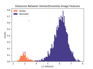
As a quick way to compare different models without getting confused by a multitude of histograms, we will take the percentage of distances that fall above each threshold. The closer to zero, the better. This can be readily put in tabular form for easy perusal.
Analysis
To get an idea of how the model’s feature vector breaks down, we do a principle component analysis of the model’s feature space. This can be done by calculating the covariance matrix for the feature vectors calculated from a set of images - resulting in a [1792x1792] matrix. The covariance matrix is a way of measuring the cross correlations between the components of the feature vector. A SVD Decomposition of the covariance matrix will gives us the leading eigen vectors and their corresponding eigen values of the feature space - in descending order.
cov = U * $\Sigma$ * $V^T$
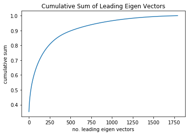
The eigen values can be found in diagonal[$\Sigma$] Plotting the cumulative sum of these eigen values:
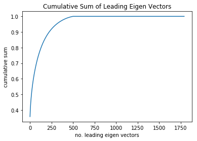
As you can see, the curve tops out at around 500 of the most significant eigen vectors. That is, most of the information in the feature vector would fit in a 500 dimensional vector, making for a compression rate of 500/1792 = 0.28. What is more is that the slope significantly slows after 250. In other words, that is the point of diminishing returns of new information that comes with each additional eigen vector.
It is important to keep in mind that memory limitations prohibit this experiment from being carried out with more than a random selection of 500 images. However, we get similar results for different random selections.
Here’s the script for how I build the pca transform model using svd decomposition: train_pca_with_svd.ipynb It relies on test images in Tensorflow’s .tfrecord format in your google drive. There’s another script in the repository for putting images in .tfrecord format.
We can use the eigen vectors from the SVD decomposition - the columns of U - to transform the feature vector into its principle componenets. We run our comparison tests on the resulting transforms for the first N coordinates - for N = 512, 256, 128, 64 and 32. So, we get a sense of how many principle components are needed for each discrimination task. Here are the results:
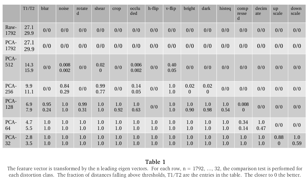
The raw feature vector, raw-1792, and the full pca transform, pca-1792, do indeed appear to be pretty good descriptors for the image content, at least according to this test. As expected, this ability is preserved when only the 512 leading eigen vectors are kept, the only category that fails being the vertical flip. Although it is somewhat curious that the horizontal flip distortion remains good. By pca-256, it fails in noise, shear, occlusion with text overlay, and, of course, vertical flip, which shows there’s some crucial information in those dropped eigen vectors for those categories. Notice how the metric steadily degrades going down the columns.
Analasis UPDATE
It turns out that using more images to compute the covariance matrix - upon which the svd decomposition is based - does indeed change the above cumulative sum plot of eigen values. Here is the plot for 4000 images:
As you can see, while the overall shape of the plot remains the same - that is, the point of diminishing returns is still reached at around 250 leading eigenvectors - there is more variance in the smaller eigenvectors. This would explain why the ability to discriminate with respect to such distortion as vertical flipping is lost with as few as 500 leading eigenvectors.
Fortunately, it doesn’t appear to have changed the results of our test:
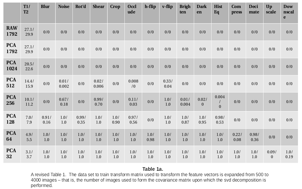
As a matter of fact, if anything, there appears to be some modest improvements.
Training Linear PCA models On a Large Set of Images
Next, we train on a larger set of images. We use images from the mirflickr25k data set of 25,000 images. There’s a script in the repository to put them in Tensorflow’s .tfrecord format. For taining, we break the image set down as follows: 20,000 for training set, 2,000 for validation set, and 3,000 for a test set.
The model used is an autoencoder trained to learn a mapping from a 1792-dimension feature vector to a 256-dimension descriptor. The new layers of the autoencoder model can be summarized like so:
h = $\sigma$(Wf + b1)
y = $W^T$h + b2
for weights, W and bias vectors, b1 and b2. f is the feature vector, h the hidden layer and y the reconstruction of f. $\sigma$(.) is the transfer function. We try three different variants of a transfer function: linear identity, non-linear sigmoid activation, and a non-linear relu activation.
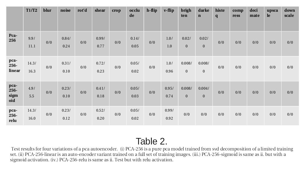
The top row is merely a repeat from the above results from the svd decomposition. The important takeaway here is that all three models, trained on the full set of 20k images, get some improvement over the first row on this test. Even the pca-256-linear strictly linear auto-encoder model appears to gain some advantage. The non-linearities introduced by the sigmoid and relu activation functions offer additional benefit.
libpHash Results
To give us some indication for how these results stack up, we put our earlier developed perceptual hashes to the test.
| pHash | description | length | distance metric |
|---|---|---|---|
| dctimage | DCT transform | 64-bit | hamming distance |
| radial | Radon transform | 180-byte | peak cross correlation |
| bmb | block mean bit | 256-bit | hamming distance |
| mh | mexican hat wavelet | 1024-bit | hamming distance |
An important distinction is that these perceptual hashes are much more concise than the above derived descriptors. Properly quantized, the pca-256 would be 256 bytes long, which would be 2k bits. Also, they are completely deterministic and not derived from any machine learning techniques whatsoever.
Results:
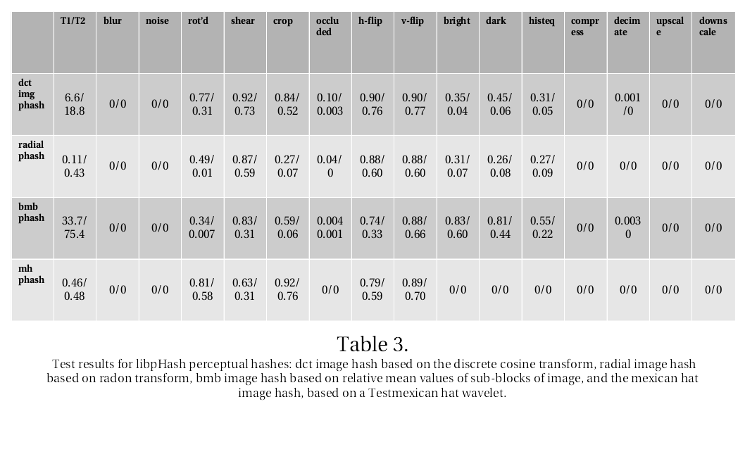
Quite an improvement compared to the old hashes. Though sufficient in certain areas - like blur, noise, occlusion
with text overlay, compression, decimation, upscale and downscale - there are serious deficiencies in the others.
It is noteworthy that the MH image hash is far superior in the bright, dark and histeq categories.
Ideas For Other Post
-
Explore other models.
-
multiple layer auto-encoder. Try adding layers so as to diminish the features gradually. Like three layers 1792->1024->512->256 with a sigmoid activation in each layer. However, my efforts so far have met with limited success in this area - at least, in terms of this testing procedure.
-
Contractive Auto-encoder. Add a Jacobian norm as a regularization term to the learning process. The Jacobian matrix is a matrix of first derivatives of the hidden layer with respect to the weights. Its norm is a measure of rate of change of the hidden layer. A regularization term should theoretically smooth the area around the immediate vicinity of each training sample.
I’ll leave it at that for this post. Questions or comments can be sent to me at Contact
Or simply reply in the issues on github: Comments and Suggestions